Examples
Refractive index and radius determination
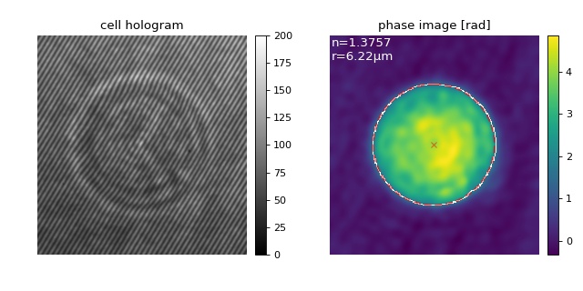
OPD edge-detection approach with a single cell
This example illustrates how qpsphere can be used to determine
the radius and the refractive index of a spherical cell.
The hologram of the myeloid leukemia cell (HL60) on the left was
recorded using digital holographic microscopy (DHM).
In the quantitative phase image on the right, the detected cell
contour (white) and the subsequent circle fit (red) as well as the
resulting average radius and refractive index of the cell
are shown. The setup used for recording these data is described in
[SSM+15] which also contains a description of the
basic steps to determine the position and radius of the cell and
to subsequently compute the average refractive index from the
experimental phase data. The experimental data is loaded and
background-corrected using qpimage.
 1import matplotlib
 2import matplotlib.pylab as plt
 3import numpy as np
 4import qpimage
 5import qpsphere
 6
 7# load the experimental data
 8edata = np.load("./data/hologram_cell.npz")
 9
10# create QPImage instance
11qpi = qpimage.QPImage(data=edata["data"],
12                      bg_data=edata["bg_data"],
13                      which_data="hologram",
14                      meta_data={"wavelength": 633e-9,
15                                 "pixel size": 0.107e-6,
16                                 "medium index": 1.335
17                                 }
18                      )
19
20# background correction
21qpi.compute_bg(which_data=["amplitude", "phase"],
22               fit_offset="fit",
23               fit_profile="tilt",
24               border_px=5,
25               )
26
27# determine radius and refractive index, guess the cell radius: 10µm
28n, r, (cx, cy), edge = qpsphere.edgefit.analyze(qpi=qpi,
29                                                r0=10e-6,
30                                                ret_center=True,
31                                                ret_edge=True)
32
33# plot results
34fig = plt.figure(figsize=(8, 4))
35matplotlib.rcParams["image.interpolation"] = "bicubic"
36holkw = {"cmap": "gray",
37         "vmin": 0,
38         "vmax": 200}
39# hologram image
40ax1 = plt.subplot(121, title="cell hologram")
41map1 = ax1.imshow(edata["data"].T, **holkw)
42plt.colorbar(map1, ax=ax1, fraction=.048, pad=0.04)
43# phase image
44ax2 = plt.subplot(122, title="phase image [rad]")
45map2 = ax2.imshow(qpi.pha.T)
46# edge
47edgeplot = np.ma.masked_where(edge == 0, edge)
48ax2.imshow(edgeplot.T, cmap="gray_r", interpolation="none")
49# fitted circle center
50plt.plot(cx, cy, "xr", alpha=.5)
51# fitted circle perimeter
52circle = plt.Circle((cx, cy), r / qpi["pixel size"],
53                    color='r', fill=False, ls="dashed", lw=2, alpha=.5)
54ax2.add_artist(circle)
55# fitting results as text
56info = "n={:.4F}\nr={:.2f}µm".format(n, r * 1e6)
57ax2.text(.8, .8, info, color="w", fontsize="12", verticalalignment="top")
58plt.colorbar(map2, ax=ax2, fraction=.048, pad=0.04)
59# disable axes
60[ax.axis("off") for ax in [ax1, ax2]]
61
62plt.tight_layout()
63plt.show()
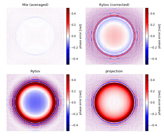
Comparison of light-scattering models
The phase error map allows a comparison of the ability of the modeling methods implemented in qpsphere to reproduce the phase delay introduced by a dielectric sphere. For a quantitative comparison, see reference [MSG+18].
 1import matplotlib.pylab as plt
 2import qpsphere
 3
 4kwargs = {"radius": 10e-6,  # 10µm
 5          "sphere_index": 1.380,  # cell
 6          "medium_index": 1.335,  # PBS
 7          "wavelength": 647.1e-9,  # krypton laser
 8          "grid_size": (200, 200),
 9          }
10
11px_size = 3 * kwargs["radius"] / kwargs["grid_size"][0]
12kwargs["pixel_size"] = px_size
13
14# mie (long computation time)
15qpi_mie = qpsphere.simulate(model="mie", **kwargs)
16
17# mie averaged
18qpi_mie_avg = qpsphere.simulate(model="mie-avg", **kwargs)
19
20# rytov corrected
21qpi_ryt_sc = qpsphere.simulate(model="rytov-sc", **kwargs)
22
23# rytov
24qpi_ryt = qpsphere.simulate(model="rytov", **kwargs)
25
26# projection
27qpi_proj = qpsphere.simulate(model="projection", **kwargs)
28
29kwargs = {"vmin": -.5,
30          "vmax": .5,
31          "cmap": "seismic"}
32
33plt.figure(figsize=(8, 6.8))
34
35ax1 = plt.subplot(221, title="Mie (averaged)")
36pmap = plt.imshow(qpi_mie.pha - qpi_mie_avg.pha, **kwargs)
37
38ax2 = plt.subplot(222, title="Rytov (corrected)")
39plt.imshow(qpi_mie.pha - qpi_ryt_sc.pha, **kwargs)
40
41ax3 = plt.subplot(223, title="Rytov")
42plt.imshow(qpi_mie.pha - qpi_ryt.pha, **kwargs)
43
44ax4 = plt.subplot(224, title="projection")
45plt.imshow(qpi_mie.pha - qpi_proj.pha, **kwargs)
46
47# disable axes
48for ax in [ax1, ax2, ax3, ax4]:
49    ax.axis("off")
50    plt.colorbar(pmap, ax=ax, fraction=.045, pad=0.04,
51                 label="phase error [rad]")
52
53plt.tight_layout(w_pad=0, h_pad=0)
54plt.show()
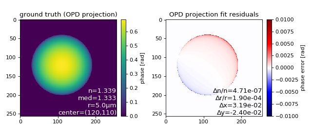
OPD projection image fit applied to an OPD simulation
This examples illustrates how the refractive index and radius of a sphere can be determined using the 2D (image-based) phase fitting algorithm.
 1import matplotlib.pylab as plt
 2
 3import qpsphere
 4
 5# run simulation with projection model
 6r = 5e-6
 7n = 1.339
 8med = 1.333
 9c = (120, 110)
10qpi = qpsphere.simulate(radius=r,
11                        sphere_index=n,
12                        medium_index=med,
13                        wavelength=550e-9,
14                        grid_size=(256, 256),
15                        model="projection",
16                        center=c)
17
18# fit simulation with projection model
19n_fit, r_fit, c_fit, qpi_fit = qpsphere.analyze(qpi=qpi,
20                                                r0=4e-6,
21                                                method="image",
22                                                model="projection",
23                                                imagekw={"verbose": 1},
24                                                ret_center=True,
25                                                ret_qpi=True)
26
27# plot results
28fig = plt.figure(figsize=(8, 3.5))
29txtkwargs = {"verticalalignment": "bottom",
30             "horizontalalignment": "right",
31             "fontsize": 12}
32
33ax1 = plt.subplot(121, title="ground truth (OPD projection)")
34map1 = ax1.imshow(qpi.pha)
35plt.colorbar(map1, ax=ax1, fraction=.046, pad=0.04, label="phase [rad]")
36t1 = "n={:.3f}\nmed={:.3f}\nr={:.1f}µm\ncenter=({:d},{:d})".format(
37    n, med, r * 1e6, c[0], c[1])
38ax1.text(1, 0, t1, transform=ax1.transAxes, color="w", **txtkwargs)
39
40ax2 = plt.subplot(122, title="OPD projection fit residuals")
41map2 = ax2.imshow(qpi.pha - qpi_fit.pha, vmin=-.01, vmax=.01, cmap="seismic")
42plt.colorbar(map2, ax=ax2, fraction=.046, pad=0.04, label="phase error [rad]")
43t2 = "Δn/n={:.2e}\nΔr/r={:.2e}\nΔx={:.2e}\nΔy={:.2e}".format(
44    abs(n - n_fit) / n, abs(r - r_fit) / r,
45    c_fit[0] - c[0], c_fit[1] - c[1])
46ax2.text(1, 0, t2, transform=ax2.transAxes, color="k", **txtkwargs)
47
48plt.tight_layout()
49plt.show()
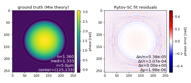
Rytov-SC image fit applied to a Mie simulation
This examples illustrates how the refractive index and radius of a sphere can be determined accurately using the 2D phase fitting algorithm with the systematically corrected Rytov approximation.
 1import matplotlib.pylab as plt
 2
 3import qpsphere
 4
 5# run simulation with averaged Mie model
 6r = 5e-6
 7n = 1.360
 8med = 1.333
 9c = (125, 133)
10qpi = qpsphere.simulate(radius=r,
11                        sphere_index=n,
12                        medium_index=med,
13                        wavelength=550e-9,
14                        grid_size=(256, 256),
15                        model="mie-avg",
16                        center=c)
17
18# Fitting Mie simulations with the systematically corrected Rytov
19# approximation (`model="rytov sc"`) yields lower parameter errors
20# compared to the non-corrected Rytov approximation (`model="rytov"`).
21n_fit, r_fit, c_fit, qpi_fit = qpsphere.analyze(qpi=qpi,
22                                                r0=4e-6,
23                                                method="image",
24                                                model="rytov-sc",
25                                                imagekw={"verbose": 1},
26                                                ret_center=True,
27                                                ret_qpi=True)
28
29# plot results
30fig = plt.figure(figsize=(8, 3.5))
31txtkwargs = {"verticalalignment": "bottom",
32             "horizontalalignment": "right",
33             "fontsize": 12}
34
35ax1 = plt.subplot(121, title="ground truth (Mie theory)")
36map1 = ax1.imshow(qpi.pha)
37plt.colorbar(map1, ax=ax1, fraction=.046, pad=0.04, label="phase [rad]")
38t1 = "n={:.3f}\nmed={:.3f}\nr={:.1f}µm\ncenter=({:d},{:d})".format(
39    n, med, r * 1e6, c[0], c[1])
40ax1.text(1, 0, t1, transform=ax1.transAxes, color="w", **txtkwargs)
41
42ax2 = plt.subplot(122, title="Rytov-SC fit residuals")
43map2 = ax2.imshow(qpi.pha - qpi_fit.pha, vmin=-.5, vmax=.5, cmap="seismic")
44plt.colorbar(map2, ax=ax2, fraction=.046, pad=0.04, label="phase error [rad]")
45t2 = "Δn/n={:.2e}\nΔr/r={:.2e}\nΔx={:.2e}\nΔy={:.2e}".format(
46    abs(n - n_fit) / n, abs(r - r_fit) / r,
47    c_fit[0] - c[0], c_fit[1] - c[1])
48ax2.text(1, 0, t2, transform=ax2.transAxes, color="k", **txtkwargs)
49
50plt.tight_layout()
51plt.show()
Other examples
Background correction based on the mask image determined with the convenience method
qpsphere.cnvnc.bg_phase_mask_for_qpi().